Air Quality and Health and Welfare
2.10 Methodologies and State of the Art for Quantifying the Health Impacts of Air Pollution
2.10.3 Approximating the Health Benefits of a Control Policy with Limited Information
2.10.3.1 Approximating the Health Benefits of a Control Policy with Limited Information
It can be very useful to quantify the benefits of a control measure in terms of improved health to the community. Quantifying health benefits can indicate how much the air pollution regulations (or lack of) contribute to loss of life, change in quality of life due to illness, loss of work product due to sick days, as well as yield quantification of the health costs and other indirect costs of air pollution. These data can help to promote regulations and demonstrate that costly controls actually may be cost effective when all factors are considered. However, this type of analysis is no small task; to complete a rigorous analysis requires detailed knowledge of where and how much of specified emissions originate, understanding of how they disperse in the atmosphere and ultimately determining how much is inhaled by different population groups. Exposure analysis, emissions measurements, air quality modeling, population tracking, age distribution, hospital records, and air quality measurements over many years are required to complete a rigorous analysis of the change in air pollution levels and resulting impacts on the community. Some very in-depth analysis has been done in the US (Hall, 2007), as well as studies elsewhere (Ho, 2007).
However, the cost and duration of such an analysis is not feasible for many situations. As an alternative, it is possible to do a simplified analysis that requires reduced input data by making use of previous studies that relate the changes in pollution to changes in health effects. This simplified approach is discussed in the following paragraphs. It is recommended only as a first step to get an overall qualitative picture of the benefits or impacts of air pollution changes. While this approach has many uncertainties, it can provide useful information in a qualitative sense when informing the public, informing policy makers, or trying to weigh the true economic costs of rules in the absence of other data. There are four steps in the simplified process in order to carry out a health benefit analysis, which are described below. The examples used in the descriptions below use particulate matter (PM) to illustrate the process, but the same approach and equations can be used for ozone or other pollutants if the relevant health related information can be found.
Step 1. Determine the relationship between pollution levels and health effects (β)
Step 2. Determine the number of cases of health effects in the baseline case (H0)
Step 3. Determine the change in ambient pollution levels due to the control (ΔA)
Step 4. Apply the exposure function to calculate the change in health impacts due to the control measures. (ΔH)
2.10.3.2 Determine the relationship between pollution levels and health effects (Step 1)
For each pollutant, there are multiple adverse health effects from the breathing of the pollutant. Some of these are acute, meaning short-term effects, and some are chronic. With acute health effects it is much easier to track the causal mechanism, and most health effects focus on these acute effects, as is the case in this section. An example of an acute effect is an asthma attack, breathing loss, or premature death due to a spike in air pollution levels over a few days or weeks. An example of a chronic effect is lung cancer, which may take lower level of exposure over decades to develop. Since chronic health effects are not considered in the described analysis, it is possible, that the health benefits of a control measure are underestimated.
The relationship between pollution and the health effects are often referred to as the Dose-Response (DR) relationship. The dose is the amount of pollution that is inhaled by the population, and the response is the number of the population that will develop the health effect. In most health literature, the Dose–Response coefficient (β) are reported which relate change in pollution levels to the increased odds of developing various health effects. The U.S. EPA defines the Dose-Response coefficient in the following manner:
Another way to describe the DR coefficient is the rate at which the population will acquire additional health impacts for every dose of pollution inhaled. There is an extraordinary amount of research and study that must go into developing DR relationships. Most DR relationships are developed from studies that track the measurements of pollutants over time with the rate of hospital records, after taking into consideration smoking and other co-founding effects. While the scientific community agrees that there is much uncertainty in using and extrapolating the DR coefficients to other situations, there are definite similarities in health effects to human beings around the world, which makes this approach reasonable as a first step.
A discussion of how to conduct an epidemiological study is not included in this text. Instead, the reader is referred to Environmental and Occupational Medicine By William N. Rom, Steven B. Markowitz or the Health Effects of Transport-related Air Pollution By Michal Krzyzanowski, Birgit Kuna-Dibbert, Jürgen Schneid. In this discussion, it is assumed that the reader does not have the time and resources to conduct a rigorous study. As an alternative, common values from the literature that are used in health impact analysis around the world for PM10 are listed in table 2.10.3-2 below. The specific health studies used to develop these β values are described further in the referenced articles. For a first cut analysis, the values listed here can be applied to any region in the world, providing that region exceeds the Ambient Air Quality Standards for that pollutant. If the region does not exceed the health based standard, this equation does not apply, and there is expected, based on present studies, to be minimal health impacts due to pollution. The values shown do not represent an exhaustive list, but are intended to provide the reader with some useful information to begin their analysis. More site specific or additional data may exist for specific areas.
Step 1 Summary: There are two methods for estimating the Dose-Response relationship:
A. Conduct Epidemiological Studies
B. Select existing DR values such as the ones shown in table 2.10.3-2 above.
2.10.3.3 Gather necessary population data (Step 2)
For estimating the end result of the number of avoided health cases, you need to determine the initial number of affected individuals. However, if this data is not collected, a simple percentage of change in health cases can be determined. A final calculation in Step 4 below will be conducted using each of these approaches. There are several steps in determining the overall baseline number of cases (H0) for each type of health effect:
1. Determine the spatial region to be assessed. Usually, this is an air basin, a metropolitan area, a county, or a state that is typically used as a boundary for air quality analysis. It can also be a smaller community, or a populated region near a facility or roadway. Thus, the number of persons impacted can vary from thousands to many millions. The extent of the area under consideration will impact the ambient effect of increasing or reducing emissions into the air. It is necessary for the selected spatial region to be the same region that the ambient air quality data is applied to, since the change in pollution levels will be calculated from the ambient monitoring data. It is also useful to have a political boundary since population data is usually gathered by political boundaries. A note of caution, it is wise to limit the boundaries to areas with similar air quality levels. This will lead to a more accurate analysis of health impacts. Typically, urban areas and sub-urban areas have differing levels of pollution, and therefore a separate analysis is conducted for sub-urban areas and urban areas if this is the case.
2. Determine the overall population living in the spatial region selected and break up the population by age group.
3. Determine the baseline rate of incidents of the health effect. Not all the DR functions are developed for the entire population, meaning the baseline population is not necessarily the entire population. For example, scientists may develop a relationship specifically linking mortality rate from PM pollution with only the adult population. Or, a relationship can be developed that relates asthma attacks with the asthmatic population. Therefore, the baseline population to apply to the mortality function would be the adult population if this were the case, and the baseline population for the asthma attacks would be the total asthmatic population. The fraction of the total population the DR applies to is referred in this text by the symbol f. The baseline population H0 is equal to the total population multiplied by the fraction f. In some instances the baseline population is the total population, therefore, f is equal to 1 in this case. Table 2.10.3-3 below lists a description of the population referred to for each of the health effects references in the earlier table 2.10.3-2 discussed along with an example of how to estimate that population.
Summary: There are several options to the user to obtain appropriate population data:
a. Use hospital records, census information to develop baseline affected population for each health effect.
b. Do not use this parameter, report the change in cases as a percentage, H0/ ΔH.
2.10.3.4 Calculate change in ambient pollution levels due to control measures under investigation (Step 3)
This is one of the more difficult steps in the process. The ultimate goal of this part of the analysis is to determine how many avoided health effects will come from applying a set of control measures that reduce emissions. Unfortunately, it is normally not readily discernable what effect a specified emissions reduction will have on the ambient concentration. Several methods are discussed below.
Air Quality Modeling: The use of ambient pollution data and air quality modeling is the preferred method and most accurate for this type of analysis. Air quality modeling can be used to estimate the change in pollution levels in different regions from the application of a single or group of control measures. This requires very sophisticated modeling for PM (if secondary particulates are important) and for Ozone as well as baseline measurements of pollution. It also requires a robust emissions inventory, meteorological input data, and changes in emissions as a result of the controls. When large uncertainties exist with the input data, it is not recommended that this modeling approach be used.
Source-Receptor Modeling: The second option is to use a source-receptor model, to calculate the levels of pollution at a certain population center due to the emissions at a specific power plant, roadway, or other emissions source. The advantage of this approach is that an intake fraction (discussed in more detail later) can explicitly track the individual effects of a certain source and specify those effects on different nearby populations. The difficulty with this approach is that it requires the use of dispersion models, detailed emissions information on when, how, and exactly where emissions are released, as well as detailed information about the meteorology, such as wind patterns and nearby topography. Another difficulty with this approach is that dispersion models do not take into consideration the effects of chemistry, secondary pollutants, such as ozone and secondary PM formation are difficult to assess using this method. The source –receptor model is often used to calculate the intake fraction for a location, which is the fraction of the pollutant that was released that is inhaled by the population. If an intake fraction exists for the source and the area under investigation, using this intake fraction is an alternative option (see later discussion).
While the above approaches are preferred and more accurate method for determining the effect on ambient pollution levels, they are useless if accurate data on the emissions and meteorology and population distribution are not available. Therefore, there are two somewhat similar alternative approaches. One is referred to as rollback modeling. The other is referred to as a box model. In both cases, the emissions and the pollution levels are assumed to be linearly proportional to changes in emissions. It should be understood that air pollution levels may not be linearly proportional to ambient air quality levels and this approach can lead to erroneous results. However, if meteorology and atmospheric chemistry are held constant, then air quality levels are often linearly related to emission rates; and thus these approaches are commonly used when a more complex model cannot be implemented.
Rollback: Usually, a region has an idea of the amount of pollution desired to be reduced or actually reduced in an air quality management program. Also, it has an idea of the current ambient levels of pollution. A simple estimate of the change in pollution levels with an estimated change in emissions levels can then be calculated. When more data exists about the spatial release of emissions, a source receptor model should be used which will result in a better estimate than the rollback approach being described here such as described in Ho (2007).
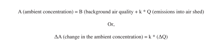
The basis for the rollback approach is the assumption that the ambient air quality in an area is linearly related to the emissions released by sources in that area. This can be written:
The critical determination in this process is the estimation of k. This can be calculated if the concentration and emissions at two different times are known. However, if not enough information exists to calculate it, a range can be used from k calculated from other areas. However, since k is a function of the region, and for PM can have secondary pollutant contributions, caution should be used in this approach. The coefficient for several known areas were calculated for several pollutants, and average results ranged from 4000-6000 ug/m3/(ton/day/km2).
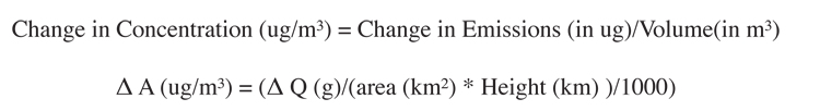
Box Model: Another simple estimate to do when no other data exists is to approximate the change in concentration by using a simple box model. The idea of a box model is simple. If you imagine the city or region and the air above it as a box, where any pollutant is introduced into the box and the pollutant is spread throughout the box evenly, then the concentration in the box is easily estimated if one knows the dimensions of the box. Again, caution should be used in this assessment because the height of the mixing layer is always changing and is region-dependent, and the assumption that the pollution is evenly mixed in the atmosphere is not ever true. In addition, this method makes no account for atmospheric reactions. The height of the mixing layer serves in the atmosphere as the top of the box, and usually ranges from 500 to 2500 meters high. The volume of the box is then simply the area of the region multiplied by the height of the mixed layer. The concentration can be calculated by:
The emissions and the changes in emissions need to be estimated for the length of time that the air is in the city. The time for which the air is in the city can be estimated by the average wind speed (assumed here to be 2 m/s) by the distance traveled over the city, which could be assumed here to be the square root of the area of the city if no other data exists. Therefore the emissions are:
Use of Air Quality Data: If the analysis is to be done looking at a historical perspective, actual changes in air quality based on air quality measurements can be used to estimate changes without special modeling or resorting to estimates of emission changes. In this case, it is important that care be taken to average out meteorological conditions that make a difference from year to year. Many times, 3 years of data is averaged together to obtain a more relevant (meteorologically neutral) air pollution level based on a least square fit to get an average trend. Also, in making averages, data from the same monitors should be used. If impacts of one variable is desired, in contrast to all the changes, the emissions change fraction of that particular variable should be applied to the overall change in pollution levels.
Summary: For estimating the impact of a future emissions change in pollution levels, there are several approaches, in order of descending complexity and accuracy:
a. Use an air quality model
b. Use Source-Receptor (or Intake Fraction) Models
c. Use a Simple Rollback Model and/or Box Model
d. Use historical ambient air quality data
2.10.3.5 Calculate change in Health Outcomes (Step 4)
To relate changes in air quality to changes in health effects, the following equation is typically used (“The Benefits and Costs of the Clean Air Act, 1999):
where:
ΔH = change in the number of cases (of a particular health outcome)
H0 = the population baseline or number of baseline cases associated with the health outcome
ΔA = the change in ambient pollution concentrations
β = the Dose-Response coefficient
For most cases where small changes in pollution are observed, the equation above is the same as ΔH =H0* β* ΔA, which is frequently shown in the literature.
For this equation, the dose response coefficient is tied to a population and an averaging of ambient pollutant levels. Care must be taken to ensure that the appropriate variables are used that correspond to the dose-response used. For example, if a β of .0025 for the asthmatic population is given, correlating to the 24-hour PM concentration, care must be taken to ensure H0 is the baseline number of asthmatics and ΔA is the change in the 24 hour (as opposed to annual) concentration. This note of caution also holds true when using an intake fraction derived in another study and applying it here.
2.10.3.6 Use of Intake Fractions in Place of Concentration Changes
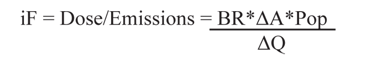
A similar but alternative approach to estimating health impacts is the use of what is commonly referred to as an “Intake fraction.” An intake fraction is defined as the fraction of emissions being released that are ingested by the population. A simple derivation from the equations used in the preceding discussions is demonstrated here to illustrate how to use an intake fraction. In this derivation, only one location and health effect and population is assumed. However, the derivation achieves the same result as when a full-fledged derivation is done. The intake fraction is normally designated as iF.
The relationship between health effects and pollutant concentrations are described as:
Or
The definition of the intake fraction is:
Where: Pop is total population,
iF is intake fraction,
BR is breathing rate,
ΔQ is emissions
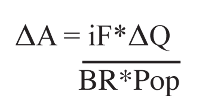
Rearranging equation 2.10.3-11 to solve for the change in ambient concentrations gives:
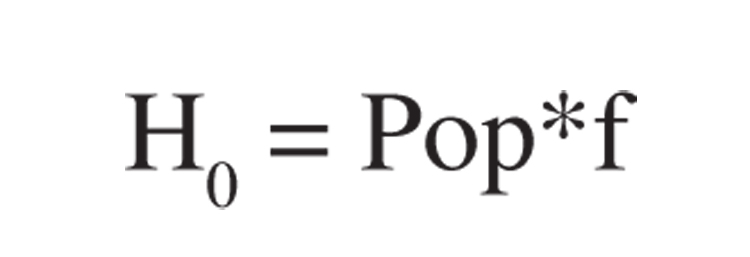
A final definition relating the population affected with the total population is:
Where: f is a fraction of the total population for specific health effect.
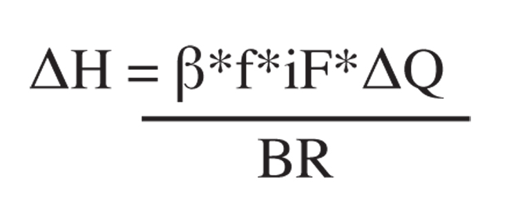
By combining equations 2.10.3-11, 2.10.3-12, and 2.10.3-9 you derive the health effects as a function of iF:
Now, the proper equations have been developed to calculate the change in health impacts given either the intake fraction or the change in concentration. Notice, using the intake fraction from equation 2.10.3-13 to estimate health effects, neither the population nor the concentration is required. This is because the development of the intake fraction has already taken this into consideration.
It can be very useful to quantify the benefits of a control measure in terms of improved health to the community. Quantifying health benefits can indicate how much the air pollution regulations (or lack of) contribute to loss of life, change in quality of life due to illness, loss of work product due to sick days, as well as yield quantification of the health costs and other indirect costs of air pollution. These data can help to promote regulations and demonstrate that costly controls actually may be cost effective when all factors are considered. However, this type of analysis is no small task; to complete a rigorous analysis requires detailed knowledge of where and how much of specified emissions originate, understanding of how they disperse in the atmosphere and ultimately determining how much is inhaled by different population groups. Exposure analysis, emissions measurements, air quality modeling, population tracking, age distribution, hospital records, and air quality measurements over many years are required to complete a rigorous analysis of the change in air pollution levels and resulting impacts on the community. Some very in-depth analysis has been done in the US (Hall, 2007), as well as studies elsewhere (Ho, 2007).
However, the cost and duration of such an analysis is not feasible for many situations. As an alternative, it is possible to do a simplified analysis that requires reduced input data by making use of previous studies that relate the changes in pollution to changes in health effects. This simplified approach is discussed in the following paragraphs. It is recommended only as a first step to get an overall qualitative picture of the benefits or impacts of air pollution changes. While this approach has many uncertainties, it can provide useful information in a qualitative sense when informing the public, informing policy makers, or trying to weigh the true economic costs of rules in the absence of other data. There are four steps in the simplified process in order to carry out a health benefit analysis, which are described below. The examples used in the descriptions below use particulate matter (PM) to illustrate the process, but the same approach and equations can be used for ozone or other pollutants if the relevant health related information can be found.
Step 1. Determine the relationship between pollution levels and health effects (β)
Step 2. Determine the number of cases of health effects in the baseline case (H0)
Step 3. Determine the change in ambient pollution levels due to the control (ΔA)
Step 4. Apply the exposure function to calculate the change in health impacts due to the control measures. (ΔH)
2.10.3.2 Determine the relationship between pollution levels and health effects (Step 1)
For each pollutant, there are multiple adverse health effects from the breathing of the pollutant. Some of these are acute, meaning short-term effects, and some are chronic. With acute health effects it is much easier to track the causal mechanism, and most health effects focus on these acute effects, as is the case in this section. An example of an acute effect is an asthma attack, breathing loss, or premature death due to a spike in air pollution levels over a few days or weeks. An example of a chronic effect is lung cancer, which may take lower level of exposure over decades to develop. Since chronic health effects are not considered in the described analysis, it is possible, that the health benefits of a control measure are underestimated.
The relationship between pollution and the health effects are often referred to as the Dose-Response (DR) relationship. The dose is the amount of pollution that is inhaled by the population, and the response is the number of the population that will develop the health effect. In most health literature, the Dose–Response coefficient (β) are reported which relate change in pollution levels to the increased odds of developing various health effects. The U.S. EPA defines the Dose-Response coefficient in the following manner:

Another way to describe the DR coefficient is the rate at which the population will acquire additional health impacts for every dose of pollution inhaled. There is an extraordinary amount of research and study that must go into developing DR relationships. Most DR relationships are developed from studies that track the measurements of pollutants over time with the rate of hospital records, after taking into consideration smoking and other co-founding effects. While the scientific community agrees that there is much uncertainty in using and extrapolating the DR coefficients to other situations, there are definite similarities in health effects to human beings around the world, which makes this approach reasonable as a first step.
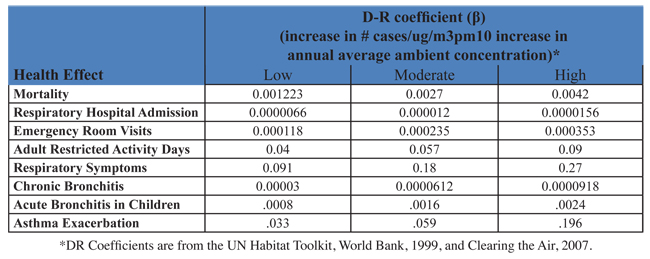
A discussion of how to conduct an epidemiological study is not included in this text. Instead, the reader is referred to Environmental and Occupational Medicine By William N. Rom, Steven B. Markowitz or the Health Effects of Transport-related Air Pollution By Michal Krzyzanowski, Birgit Kuna-Dibbert, Jürgen Schneid. In this discussion, it is assumed that the reader does not have the time and resources to conduct a rigorous study. As an alternative, common values from the literature that are used in health impact analysis around the world for PM10 are listed in table 2.10.3-2 below. The specific health studies used to develop these β values are described further in the referenced articles. For a first cut analysis, the values listed here can be applied to any region in the world, providing that region exceeds the Ambient Air Quality Standards for that pollutant. If the region does not exceed the health based standard, this equation does not apply, and there is expected, based on present studies, to be minimal health impacts due to pollution. The values shown do not represent an exhaustive list, but are intended to provide the reader with some useful information to begin their analysis. More site specific or additional data may exist for specific areas.
2.10.3-2 Accepted Risk Factors for PM10 used in Health Impact Analysis around the World

Step 1 Summary: There are two methods for estimating the Dose-Response relationship:
A. Conduct Epidemiological Studies
B. Select existing DR values such as the ones shown in table 2.10.3-2 above.
2.10.3.3 Gather necessary population data (Step 2)
For estimating the end result of the number of avoided health cases, you need to determine the initial number of affected individuals. However, if this data is not collected, a simple percentage of change in health cases can be determined. A final calculation in Step 4 below will be conducted using each of these approaches. There are several steps in determining the overall baseline number of cases (H0) for each type of health effect:
1. Determine the spatial region to be assessed. Usually, this is an air basin, a metropolitan area, a county, or a state that is typically used as a boundary for air quality analysis. It can also be a smaller community, or a populated region near a facility or roadway. Thus, the number of persons impacted can vary from thousands to many millions. The extent of the area under consideration will impact the ambient effect of increasing or reducing emissions into the air. It is necessary for the selected spatial region to be the same region that the ambient air quality data is applied to, since the change in pollution levels will be calculated from the ambient monitoring data. It is also useful to have a political boundary since population data is usually gathered by political boundaries. A note of caution, it is wise to limit the boundaries to areas with similar air quality levels. This will lead to a more accurate analysis of health impacts. Typically, urban areas and sub-urban areas have differing levels of pollution, and therefore a separate analysis is conducted for sub-urban areas and urban areas if this is the case.
2. Determine the overall population living in the spatial region selected and break up the population by age group.
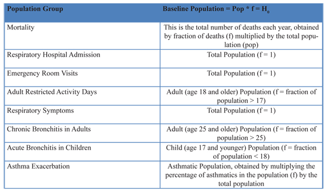
3. Determine the baseline rate of incidents of the health effect. Not all the DR functions are developed for the entire population, meaning the baseline population is not necessarily the entire population. For example, scientists may develop a relationship specifically linking mortality rate from PM pollution with only the adult population. Or, a relationship can be developed that relates asthma attacks with the asthmatic population. Therefore, the baseline population to apply to the mortality function would be the adult population if this were the case, and the baseline population for the asthma attacks would be the total asthmatic population. The fraction of the total population the DR applies to is referred in this text by the symbol f. The baseline population H0 is equal to the total population multiplied by the fraction f. In some instances the baseline population is the total population, therefore, f is equal to 1 in this case. Table 2.10.3-3 below lists a description of the population referred to for each of the health effects references in the earlier table 2.10.3-2 discussed along with an example of how to estimate that population.
2.10.3-3 Population Group to Apply to the Health Effects listed in table 2.10.3-2
Summary: There are several options to the user to obtain appropriate population data:
a. Use hospital records, census information to develop baseline affected population for each health effect.
b. Do not use this parameter, report the change in cases as a percentage, H0/ ΔH.
2.10.3.4 Calculate change in ambient pollution levels due to control measures under investigation (Step 3)
This is one of the more difficult steps in the process. The ultimate goal of this part of the analysis is to determine how many avoided health effects will come from applying a set of control measures that reduce emissions. Unfortunately, it is normally not readily discernable what effect a specified emissions reduction will have on the ambient concentration. Several methods are discussed below.
Air Quality Modeling: The use of ambient pollution data and air quality modeling is the preferred method and most accurate for this type of analysis. Air quality modeling can be used to estimate the change in pollution levels in different regions from the application of a single or group of control measures. This requires very sophisticated modeling for PM (if secondary particulates are important) and for Ozone as well as baseline measurements of pollution. It also requires a robust emissions inventory, meteorological input data, and changes in emissions as a result of the controls. When large uncertainties exist with the input data, it is not recommended that this modeling approach be used.
Source-Receptor Modeling: The second option is to use a source-receptor model, to calculate the levels of pollution at a certain population center due to the emissions at a specific power plant, roadway, or other emissions source. The advantage of this approach is that an intake fraction (discussed in more detail later) can explicitly track the individual effects of a certain source and specify those effects on different nearby populations. The difficulty with this approach is that it requires the use of dispersion models, detailed emissions information on when, how, and exactly where emissions are released, as well as detailed information about the meteorology, such as wind patterns and nearby topography. Another difficulty with this approach is that dispersion models do not take into consideration the effects of chemistry, secondary pollutants, such as ozone and secondary PM formation are difficult to assess using this method. The source –receptor model is often used to calculate the intake fraction for a location, which is the fraction of the pollutant that was released that is inhaled by the population. If an intake fraction exists for the source and the area under investigation, using this intake fraction is an alternative option (see later discussion).
While the above approaches are preferred and more accurate method for determining the effect on ambient pollution levels, they are useless if accurate data on the emissions and meteorology and population distribution are not available. Therefore, there are two somewhat similar alternative approaches. One is referred to as rollback modeling. The other is referred to as a box model. In both cases, the emissions and the pollution levels are assumed to be linearly proportional to changes in emissions. It should be understood that air pollution levels may not be linearly proportional to ambient air quality levels and this approach can lead to erroneous results. However, if meteorology and atmospheric chemistry are held constant, then air quality levels are often linearly related to emission rates; and thus these approaches are commonly used when a more complex model cannot be implemented.
Rollback: Usually, a region has an idea of the amount of pollution desired to be reduced or actually reduced in an air quality management program. Also, it has an idea of the current ambient levels of pollution. A simple estimate of the change in pollution levels with an estimated change in emissions levels can then be calculated. When more data exists about the spatial release of emissions, a source receptor model should be used which will result in a better estimate than the rollback approach being described here such as described in Ho (2007).
The basis for the rollback approach is the assumption that the ambient air quality in an area is linearly related to the emissions released by sources in that area. This can be written:
The critical determination in this process is the estimation of k. This can be calculated if the concentration and emissions at two different times are known. However, if not enough information exists to calculate it, a range can be used from k calculated from other areas. However, since k is a function of the region, and for PM can have secondary pollutant contributions, caution should be used in this approach. The coefficient for several known areas were calculated for several pollutants, and average results ranged from 4000-6000 ug/m3/(ton/day/km2).
Box Model: Another simple estimate to do when no other data exists is to approximate the change in concentration by using a simple box model. The idea of a box model is simple. If you imagine the city or region and the air above it as a box, where any pollutant is introduced into the box and the pollutant is spread throughout the box evenly, then the concentration in the box is easily estimated if one knows the dimensions of the box. Again, caution should be used in this assessment because the height of the mixing layer is always changing and is region-dependent, and the assumption that the pollution is evenly mixed in the atmosphere is not ever true. In addition, this method makes no account for atmospheric reactions. The height of the mixing layer serves in the atmosphere as the top of the box, and usually ranges from 500 to 2500 meters high. The volume of the box is then simply the area of the region multiplied by the height of the mixed layer. The concentration can be calculated by:
The emissions and the changes in emissions need to be estimated for the length of time that the air is in the city. The time for which the air is in the city can be estimated by the average wind speed (assumed here to be 2 m/s) by the distance traveled over the city, which could be assumed here to be the square root of the area of the city if no other data exists. Therefore the emissions are:

Use of Air Quality Data: If the analysis is to be done looking at a historical perspective, actual changes in air quality based on air quality measurements can be used to estimate changes without special modeling or resorting to estimates of emission changes. In this case, it is important that care be taken to average out meteorological conditions that make a difference from year to year. Many times, 3 years of data is averaged together to obtain a more relevant (meteorologically neutral) air pollution level based on a least square fit to get an average trend. Also, in making averages, data from the same monitors should be used. If impacts of one variable is desired, in contrast to all the changes, the emissions change fraction of that particular variable should be applied to the overall change in pollution levels.
Summary: For estimating the impact of a future emissions change in pollution levels, there are several approaches, in order of descending complexity and accuracy:
a. Use an air quality model
b. Use Source-Receptor (or Intake Fraction) Models
c. Use a Simple Rollback Model and/or Box Model
d. Use historical ambient air quality data
2.10.3.5 Calculate change in Health Outcomes (Step 4)
To relate changes in air quality to changes in health effects, the following equation is typically used (“The Benefits and Costs of the Clean Air Act, 1999):

where:
ΔH = change in the number of cases (of a particular health outcome)
H0 = the population baseline or number of baseline cases associated with the health outcome
ΔA = the change in ambient pollution concentrations
β = the Dose-Response coefficient
For most cases where small changes in pollution are observed, the equation above is the same as ΔH =H0* β* ΔA, which is frequently shown in the literature.
For this equation, the dose response coefficient is tied to a population and an averaging of ambient pollutant levels. Care must be taken to ensure that the appropriate variables are used that correspond to the dose-response used. For example, if a β of .0025 for the asthmatic population is given, correlating to the 24-hour PM concentration, care must be taken to ensure H0 is the baseline number of asthmatics and ΔA is the change in the 24 hour (as opposed to annual) concentration. This note of caution also holds true when using an intake fraction derived in another study and applying it here.
2.10.3.6 Use of Intake Fractions in Place of Concentration Changes
A similar but alternative approach to estimating health impacts is the use of what is commonly referred to as an “Intake fraction.” An intake fraction is defined as the fraction of emissions being released that are ingested by the population. A simple derivation from the equations used in the preceding discussions is demonstrated here to illustrate how to use an intake fraction. In this derivation, only one location and health effect and population is assumed. However, the derivation achieves the same result as when a full-fledged derivation is done. The intake fraction is normally designated as iF.
The relationship between health effects and pollutant concentrations are described as:

Or

The definition of the intake fraction is:
Where: Pop is total population,
iF is intake fraction,
BR is breathing rate,
ΔQ is emissions
Rearranging equation 2.10.3-11 to solve for the change in ambient concentrations gives:
A final definition relating the population affected with the total population is:
Where: f is a fraction of the total population for specific health effect.
By combining equations 2.10.3-11, 2.10.3-12, and 2.10.3-9 you derive the health effects as a function of iF:
Now, the proper equations have been developed to calculate the change in health impacts given either the intake fraction or the change in concentration. Notice, using the intake fraction from equation 2.10.3-13 to estimate health effects, neither the population nor the concentration is required. This is because the development of the intake fraction has already taken this into consideration.