Air Quality Modeling
7.2 Dispersion Modeling
7.2.2 Box Models
7.2.2.1 Theoretical Basis
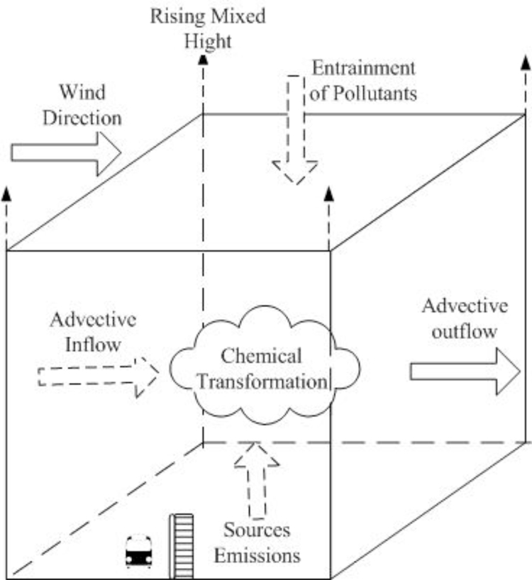
The second category of simple urban air quality models has been called box models. Figure 7.2.2-1 is a schematic diagram of a box model including source emissions near the lower boundary (surface), advective inflow and outflow to and from the sides, entrainment of pollutant from aloft due to increasing mixing height, and chemical transformations. Since uniform mixing is assumed to occur within the box whose horizontal boundaries enclose the urban area of interest, the model can predict only the volume-averaged concentration as a function of time. Diffusion from individual sources is not considered, but all sources are considered in estimating source emissions into the box. With the simplified treatment of meteorology in terms of the effective transport winds and mixing height, one can use a sophisticated chemical and photochemical module.
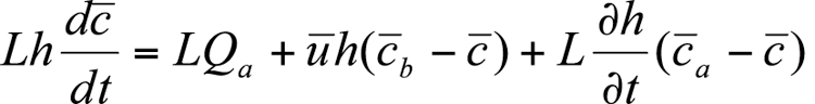
For the simplest box model without chemical transformations, one can derive a simple differential equation for the average concentration within the box from the consideration of mass conservation within the box or a slice of the box with a unit width normal to the wind flow, length L in the direction of flow, and height h equal to the mixing depth. The rate of change of mass within the box must be equal to the sum of the rates at which the pollutant mass is added by all the emission sources in the box, the change due to horizontal advection, and the change due to entrainment from the top resulting from the growth in mixing height. This can be expressed mathematically as (see e.g., Hanna et al., 1982)
where is the average concentration aloft (z > h) over the city and
  is the average background concentration upwind of the city. Equation 7.2.2-1 can be rewritten in the form
which can be solved easily for the specified values of , , ,
, , ,  , h, and
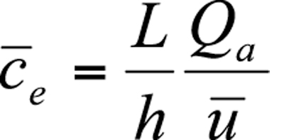
  . Further simplifications can be made for the negligible background concentrations ( = 0, = 0). Furthermore, if conditions become steady state (
 = 0, = 0), say late in the afternoon, then the equilibrium concentration is given simply by
The equilibrium or steady-state average concentration within the urban environment is directly proportional to the total rate of emission from the urban area and inversely proportional to the product of mean wind speed and mixing height, also known as the ventilation factor.
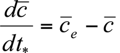
If one defines a time scale as the flushing time required for the air to pass completely over the urban area and a dimensionless time
  =
=  , then 7.2.2-3 without the background concentration terms can be written as
The solution to equation 7.2.2-5 is
where is the initial value of concentration at = 0, which is larger than the equilibrium concentration. According to the above simple box model, first proposed by Lettau (1970), the concentration decreases exponentially with increasing time and approaches its equilibrium value given by equation 7.2.2-4 after a time two to three times the flushing time. Because of its simplicity, this type of box model is often used as a screening model in regulatory applications.
With appropriate accounting for chemical and photochemical transformations, photochemical box models have also been used for predicting concentrations of ozone and other photochemical pollutants in urban areas. For example, Demerjian and Schere (1979) used such a model for predicting the ozone air quality of Houston, Texas. They used equation 7.2.2-2 plus a source term representing chemical transformations. The vertical entrainment term is found to be important, because ozone is often trapped above the inversion layer over urban areas at night and is mixed down to the surface by the growing unstable or convective mixed layer the next morning. The most complicated part of the photochemical box model is the multi-step chemical kinetic mechanism. Demerjian and Schere (1979) used a thirty-six-step mechanism and found that predicted hourly averaged concentrations of hydrocarbons, NOx, CO, and ozone were within a factor of 2 of observed concentrations.
7.2.2.2 EKMA Box Models
 One variant of the photochemical box model that has been widely used for estimating ozone concentration in urban areas is the so-called EKMA (empirical kinetic modeling approach) technique (Dodge, 1977). This approach is based on the generation of ozone concentration isopleths using an ozone isopleths plotting package (OZIPP). These isopleths are three-dimensional plots of daily maximum hourly average ozone concentrations that are generated in mixtures with various initial NMHC and NOx concentrations. Figure 7.2.2-7 shows a set of such isopleths that were calculated using the EKMA approach analogous to that used in photochemical box models.
The following assumptions were made in obtaining the isopleths in figure 7.2.2-7 (Finlayson-Pitts and Pitts, 1986):
1. The hydrocarbon mix consists of propane and butane in a 1:3 ratio (as carbon), while aldehydes account for 5 percent (as carbon)of the initial NMHC.
2. Initial NO2 concentrations were 25 percent of the initial NOx concentration.
3. No addition of fresh pollutants occurred during the simulation period of 8:00 AM to 5:00 PM (local time) for the summer solstice at 34°N latitude.
4. Dilution is assumed to occur at a rate of 3 percent per hour until 3:00 PM with no dilution afterward.
5. Background or transported ozone is assumed to be negligible.
The chemical mechanism currently used in EKMA is the carbon-bond mechanism, but other mechanisms using a lumped approach can also be incorporated. These mechanisms are usually validated against the smog chamber data. The ozone isopleths in figure 7.2.2-7 illustrate the importance of both NMHC and NOx concentrations as well as of their ratio in the formulation of ozone control strategies. Ozone isopleths show a ridge along the diagonal running from the lower left to the upper right of the diagram. The predicted ozone maximum concentration increases with simultaneous increases in the initial concentrations of NMHC and NOx provided their ratio is consistent with the ridge line; for the conditions of figure 7.2.2-7 12.3 this ratio is about 6. The characteristic NMHC/NOx ratios of different urban areas will, in general, not coincide with the ridge line but will lie on one or the other side of it. The NMHC/NOx ratio has important implications for ozone control in different urban areas.
If an urban area is characterized by large NMHC emissions such that the NMHC/NOx ratio is greater than the ridge line value, the ozone isopleths run al-most parallel to the NMHC axis. Thus, the maximum O3 concentration is not very sensitive to the hydro-carbon control if NOx is kept constant. Ozone formation under these conditions is limited by the available NOx. Therefore, reducing NOx while keeping NMHC levels constant or reducing both NMHC and NOx simultaneously while keeping their ratio constant would reduce the maximum ozone concentration.
A different control strategy might be more appropriate for an urban area with smaller NMHC/NOx ratio than the ridge line value in figure 7.2.2-7. Here reducing NMHC with constant NOx would lead to significant reductions in the ozone maximum. The same can be accomplished by decreasing both NMHC and NOx simultaneously while keeping their ratio constant. However, in contrast to the situation of greater NMHC/NOx ratios, reducing NOx while keeping NMHC constant would lead to higher ozone concentrations until the ridge line is reached. Therefore, the best overall control strategy, if applied uniformly to all urban areas with significant ozone pollution, is to control both NMHC and NOx emissions. The EKMA modeling approach can play a very useful role in developing optimum control strategies for different urban areas. City-specific versions of EKMA in which ozone isopleth diagrams are generated using data more representative of particular locations and transport of pollutants from outside is also taken into account are found to be more appropriate and useful for this purpose. Some of the limitations of this approach have been discussed by Finlayson-Pitts and Pitts (1986).
The second category of simple urban air quality models has been called box models. Figure 7.2.2-1 is a schematic diagram of a box model including source emissions near the lower boundary (surface), advective inflow and outflow to and from the sides, entrainment of pollutant from aloft due to increasing mixing height, and chemical transformations. Since uniform mixing is assumed to occur within the box whose horizontal boundaries enclose the urban area of interest, the model can predict only the volume-averaged concentration as a function of time. Diffusion from individual sources is not considered, but all sources are considered in estimating source emissions into the box. With the simplified treatment of meteorology in terms of the effective transport winds and mixing height, one can use a sophisticated chemical and photochemical module.
For the simplest box model without chemical transformations, one can derive a simple differential equation for the average concentration
within the box from the consideration of mass conservation within the box or a slice of the box with a unit width normal to the wind flow, length L in the direction of flow, and height h equal to the mixing depth. The rate of change of mass within the box must be equal to the sum of the rates at which the pollutant mass is added by all the emission sources in the box, the change due to horizontal advection, and the change due to entrainment from the top resulting from the growth in mixing height. This can be expressed mathematically as (see e.g., Hanna et al., 1982)
where
is the average concentration aloft (z > h) over the city and is the average background concentration upwind of the city. Equation 7.2.2-1 can be rewritten in the form

which can be solved easily for the specified values of
, , , , h, and . Further simplifications can be made for the negligible background concentrations ( = 0, = 0). Furthermore, if conditions become steady state ( = 0, = 0), say late in the afternoon, then the equilibrium concentration is given simply by
The equilibrium or steady-state average concentration within the urban environment is directly proportional to the total rate of emission from the urban area and inversely proportional to the product of mean wind speed and mixing height, also known as the ventilation factor.
If one defines a time scale
as the flushing time required for the air to pass completely over the urban area and a dimensionless time = , then 7.2.2-3 without the background concentration terms can be written as
The solution to equation 7.2.2-5 is
where
is the initial value of concentration at = 0, which is larger than the equilibrium concentration. According to the above simple box model, first proposed by Lettau (1970), the concentration decreases exponentially with increasing time and approaches its equilibrium value given by equation 7.2.2-4 after a time two to three times the flushing time. Because of its simplicity, this type of box model is often used as a screening model in regulatory applications.
With appropriate accounting for chemical and photochemical transformations, photochemical box models have also been used for predicting concentrations of ozone and other photochemical pollutants in urban areas. For example, Demerjian and Schere (1979) used such a model for predicting the ozone air quality of Houston, Texas. They used equation 7.2.2-2 plus a source term representing chemical transformations. The vertical entrainment term is found to be important, because ozone is often trapped above the inversion layer over urban areas at night and is mixed down to the surface by the growing unstable or convective mixed layer the next morning. The most complicated part of the photochemical box model is the multi-step chemical kinetic mechanism. Demerjian and Schere (1979) used a thirty-six-step mechanism and found that predicted hourly averaged concentrations of hydrocarbons, NOx, CO, and ozone were within a factor of 2 of observed concentrations.
7.2.2.2 EKMA Box Models
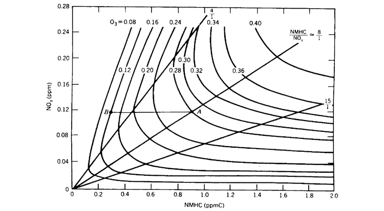
7.2.2-7 Ozone Isopleths used in the EKMA (empirical kinetic modeling approach). NMHC, non-methane hydrocarbons. From Dodge, 1997.
The following assumptions were made in obtaining the isopleths in figure 7.2.2-7 (Finlayson-Pitts and Pitts, 1986):
1. The hydrocarbon mix consists of propane and butane in a 1:3 ratio (as carbon), while aldehydes account for 5 percent (as carbon)of the initial NMHC.
2. Initial NO2 concentrations were 25 percent of the initial NOx concentration.
3. No addition of fresh pollutants occurred during the simulation period of 8:00 AM to 5:00 PM (local time) for the summer solstice at 34°N latitude.
4. Dilution is assumed to occur at a rate of 3 percent per hour until 3:00 PM with no dilution afterward.
5. Background or transported ozone is assumed to be negligible.
The chemical mechanism currently used in EKMA is the carbon-bond mechanism, but other mechanisms using a lumped approach can also be incorporated. These mechanisms are usually validated against the smog chamber data. The ozone isopleths in figure 7.2.2-7 illustrate the importance of both NMHC and NOx concentrations as well as of their ratio in the formulation of ozone control strategies. Ozone isopleths show a ridge along the diagonal running from the lower left to the upper right of the diagram. The predicted ozone maximum concentration increases with simultaneous increases in the initial concentrations of NMHC and NOx provided their ratio is consistent with the ridge line; for the conditions of figure 7.2.2-7 12.3 this ratio is about 6. The characteristic NMHC/NOx ratios of different urban areas will, in general, not coincide with the ridge line but will lie on one or the other side of it. The NMHC/NOx ratio has important implications for ozone control in different urban areas.
If an urban area is characterized by large NMHC emissions such that the NMHC/NOx ratio is greater than the ridge line value, the ozone isopleths run al-most parallel to the NMHC axis. Thus, the maximum O3 concentration is not very sensitive to the hydro-carbon control if NOx is kept constant. Ozone formation under these conditions is limited by the available NOx. Therefore, reducing NOx while keeping NMHC levels constant or reducing both NMHC and NOx simultaneously while keeping their ratio constant would reduce the maximum ozone concentration.
A different control strategy might be more appropriate for an urban area with smaller NMHC/NOx ratio than the ridge line value in figure 7.2.2-7. Here reducing NMHC with constant NOx would lead to significant reductions in the ozone maximum. The same can be accomplished by decreasing both NMHC and NOx simultaneously while keeping their ratio constant. However, in contrast to the situation of greater NMHC/NOx ratios, reducing NOx while keeping NMHC constant would lead to higher ozone concentrations until the ridge line is reached. Therefore, the best overall control strategy, if applied uniformly to all urban areas with significant ozone pollution, is to control both NMHC and NOx emissions. The EKMA modeling approach can play a very useful role in developing optimum control strategies for different urban areas. City-specific versions of EKMA in which ozone isopleth diagrams are generated using data more representative of particular locations and transport of pollutants from outside is also taken into account are found to be more appropriate and useful for this purpose. Some of the limitations of this approach have been discussed by Finlayson-Pitts and Pitts (1986).