Estimating Emissions from Sources of Air Pollution
6.2 Estimating Emissions from On-Road Mobile Sources
6.2.5 The International Vehicle Emissions Model
6.2.5.1 Introduction
The International Vehicle Emissions model, or IVE model, as well as the EPA MOVES model, take a radical departure in their approach to making emission estimates for on-road mobile sources compared to the MOBILE, EMFAC and European Models. As noted in the previous section, most current models depend on fixed driving patterns to make their calculations and then make approximate adjustments based on roadway speeds. Both the IVE and MOVES models allow information about the driving to be input directly into the model itself and emission calculations are made based on parameters from those specific driving parameters. Driving parameters can be entered on a day or on an hour-by-hour basis, allowing specific calculation of emissions by the hour or for a specific roadway to improve atmospheric modeling efforts.
6.2.5.2 Theory of Model Operation
An important observation made by the USEPA, ISSRC, UCR, and other researchers in the early to mid-1990s is that there is a close relationship between the power (energy/sec) demand on a vehicle and the emissions that the vehicle produces. This is a logical conclusion when considered in light of combustion chemistry. The law of conservation of energy requires that a vehicle burn fuel commensurate with the energy demand on the vehicle. Thus, when more energy is demanded more fuel is burned. As discussed with 6.2.5-1 (seen in a previous section), the greater the fuel-use, the greater the amounts of other pollutants that will be formed if air/fuel ratios and other emission impacting variables are kept the same.
There have been two ways to incorporate fuel use or power demand into vehicle emissions models. The first method is a top down fuel-based emissions models that relate emissions to the amount of fuel used. Instead of a gram/distance traveled, they produce a gram/fuel consumed emission factor. Then, there is reliance on properly estimating both the emission factor and the activity (being overall fuel use). While this is a useful approach, there are some limitations of a fuel based emission factor model. These include difficulties in accounting for other (non-fuel based) parameters that can affect emissions, as well as the uncertainties in estimating the overall fuel used in vehicle applications. A second approach is to develop a bottom up physical model that predicts the emissions as a function of engine power and fuel use for a specific vehicle. This is an excellent method for accounting for the variations in emissions as a function of many parameters, including fuel use. The CMEM model is an example of a model that uses this approach. However, the drawback for using a model such as CMEM for regional scale applications is the vast amount of input data that is required. A hybrid approach to these methods is to use the fuel consumption as a parameter in how emissions vary when the vehicle operation changes. This is similar to the IVE and MOVES approach, and is described here.
A useful way to estimate fuel use is through measuring the vehicle specific power. Figure 6.2.5-2 shows the impact of vehicle power demand on vehicle CO2 and CO emissions. The x-axis shows an approximation of vehicle specific power and the y-axis shows the emissions rate in grams/second. A negative value of vehicle specific power corresponds to the vehicle decelerating.
CO2 emissions change rather linearly with respect to power demand and fuel use as would be expected. CO emissions on the other hand show a much larger change in emission rates relative to power demand. The reason for the higher CO sensitivity is because, the air/fuel mix in the engine changes to a degree as vehicles are accelerated and decelerated, especially in the case of large changes. CO2 emissions increase by a factor of 12 from the idle state to maximum power demand while CO emissions change by a factor of 250 from the idle state to maximum power demand for a catalyst controlled vehicle. For either pollutant, the way that a vehicle is operated will have significant impact on resulting emissions.
The IVE model estimates emissions by taking the fraction of time that a vehicle spends in each of 60 power demand bins and multiplying the fraction of time by an emissions adjustment factor. The 60 multiplications are then summed creating an average correction factor for that driving pattern. The emissions adjustment factors for each bin are based on test data. However, the actual adjustment factors used in the model are all normalized by multiplying the emission rates by a constant so that the driving pattern from the hot running portion of the FTP driving pattern if used with the adjustment factors will produce an overall driving correction factor of one.
Equation 6.2.5-3 indicates the calculation process to produce a driving correction factor for the IVE model.
In this case, KP[t] = overall driving correction factor for technology t, Cb[t] = driving correction adjustment for power bin b and technology t, Fb = fraction of time a vehicle spends driving in power bin b. The sum is from bin 0 to bin 59.
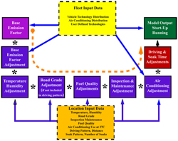
Emission estimates are further adjusted in the IVE model based on the other vehicle operating factors that impact emissions such as altitude, ambient temperature, fuel quality, and such. The proper emission adjustments for a vehicle are determined based on the vehicle operating factors and their potential interaction with one another. Figure 6.2.5-4 illustrates the calculation flow for the IVE model.
Equation 6.2.5-3 presents the mathematical equivalent for the calculation of the adjusted base emission rate represented by the blue colored boxes in 6.2.5-4.
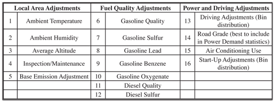
In this case, the subscript “t” refers to the vehicle technology and the number subscript refers to the various adjustment factors as outlined in table 6.2.5-6. B[t] refers to the base emission rate in the model for either start emissions or running emissions. Kp[t] refers to the adjustment factor determined from the power demand statistics shown in equation 6.2.5-3. In the case of start emissions, Kp[t] = 1 since there is no driving adjustment.
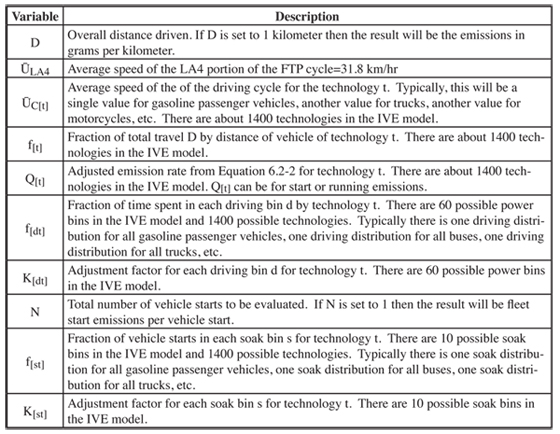
Once the adjusted base emission factor (Q[t]) is determined for each technology of interest, then the fleet start and running emissions can be calculated as shown in 6.2.5-7 and 6.2.5-8.
A description of the variables in equation 6.2.5-7 and equation 6.2.5-8 can be found in table 6.2.5-9.
Qrunning and Qstart can be calculated for each hour of the day and for each road type to be evaluated. The IVE model allows for all of these possibilities to be carried out at one time or they can be evaluated independently.
The information needed by the IVE model for fleet technology distributions is provided to the model in what is designated as a Fleet File. This can be supplied to the model as a tab delimited text file. The information needed by the IVE model for a particular location is provided to the model in what is designated as a Location File. The location file can also be supplied as a tab delimited file. The model can make use of hundreds of Fleet Files and hundreds of Location files allowing for considerable flexibility. The actual creation of Location and Fleet files can be complex. The reader is referred to the IVE Model Users Manual for more discussion. The model can be downloaded free from the internet site http://www.issrc.org/ive along with the user’s manual. The IVE model interface now includes Chinese, English, Russian, and Spanish.


